Phylogenetics — the study of evolutionary relationships between organisms — has traditionally relied on multiple sequence alignment (MSA) as a first step. While MSA works well for closely related sequences, it becomes painfully slow and computationally expensive when you scale to hundreds or thousands of sequences, especially across diverse taxa.
Covary, developed by ChordexBio, takes a different approach: it skips alignment altogether. Instead, it uses translation-aware, alignment-free embeddings powered by deep learning (via TIPs-VF) to represent and compare genetic sequences — enabling fast, scalable phylogenomic analyses. The framework is described in full in the preprint published on bioRxiv (2025).
This guide will walk you through running Covary from scratch — no prior bioinformatics experience required. All you need is a multi-FASTA file, a Google account, and about 30–60 minutes of your time.
What is Covary, and why does it matter?
At its core, Covary transforms each DNA sequence into a numerical vector — a compact mathematical representation that captures the sequence's composition, length, position, and even codon-level (translation-aware) features. These vectors can then be compared, clustered, and visualized without ever needing to align sequences to each other.
Key capabilities include:
- Alignment-free analysis — no MSA required, dramatically reducing compute time for large datasets.
- Translation-aware embeddings — biologically meaningful representations that work on both coding and non-coding sequences.
- Distance-based clustering — generates Euclidean pairwise distance matrices for downstream clustering and tree building.
- Multi-level taxonomic resolution — can distinguish sequences at species, genus, family, and order levels.
- Rich visualizations — heatmaps, dendrograms, and scatter plots (PCA, t-SNE, UMAP) out of the box.
Covary has been benchmarked on datasets including 906 whole-genome sequences of SARS-CoV-2 in a single run, with smooth performance on a GPU runtime.
Before you begin: What you will need
- A Google account (to access Google Colab)
- A multi-FASTA file of DNA sequences (see format below)
- Covary v2.1 (may require license) — no local installation required
- A GPU runtime in Colab (free T4 GPU is sufficient for most analyses)
💡 Note on RNA sequences: Covary accepts DNA sequences (A, T, C, G). If you have RNA data, convert U → T before uploading. Covary's k-mer encoder is optimized for the DNA alphabet.
Step 1 — Prepare your multi-FASTA file
Your input must be a multi-FASTA file: a plain text file where each sequence entry begins with a > header line followed by the nucleotide sequence. Here is a sample from the Covary documentation using 16S ribosomal RNA sequences of Thermus species:
>NR_181868.1 Thermus brevis strain SYSU G05001 16S ribosomal RNA, partial sequence
GACATGCAAGTCGAGCGGGGCGGGTTTATACCTGCCCAGCGGCGGACGGGTGAGTAACGC
GTGGGTGACCTACCTGGAAGAGGCGGACAACCTGGGGAAACCCAGGCTAATCCGCCATGT
GGTCCTGTCCTGTGGGGCAGGACTAAAGGGTGGATAGCCCGCTTCCGGATGGGCCCGCGT
CCCATCAGCTAGTTGGTGGGGTAAGAGCCCACCAAGGCGACGACGGGTAGCCGGTCTGAG

>NR_181790.1 Thermus brevis strain SYSU G05002 16S ribosomal RNA, partial sequence
GACATGCAAGTCGAGCGGGGCGGGTTTATACCTGCCCAGCGGCGGACGGGTGAGTAACGC
GTGGGTGACCTACCTGGAAGAGGCGGACAACCTGGGGAAACCCAGGCTAATCCGCCATGT
GGTCCTGTCCTGTGGGGCAGGACTAAAGGGTGGATAGCCCGCTTCCGGATGGGCCCGCGT
CCCATCAGCTAGTTGGTGGGGTAAGAGCCCACCAAGGCGACGACGGGTAGCCGGTCTGAG

>NR_180714.1 Thermus sediminis strain L198 16S ribosomal RNA, partial sequence
GACATGCAAGTCGTGCGGGCCGTGGGGTTTCTCACGGCTAGCGGCGGACGGGTGAGTAAC
GCGTGGGTGACCTACCCGGAAGAGGGGGACAACCTGGGGAAACCCAGGCTAATCCCCCAT
GTGGACGCATCCTGTGGGGTGCGTTCAAAGGGCGTTGCCCGCTTCCGGATGGGCCCGCGT
CCCATCAGCCAGTTGGTGGGGTAAAGGCCCACCAAGGCGACGACGGGTAGCCGGTCTGAG
Tips for preparing your FASTA file:
- Each entry must start with
>followed by a unique accession or identifier. - Remove any extra whitespace, blank lines within sequences, or non-standard characters.
- Avoid sequences with excessive ambiguous bases (
Ns) — by default, Covary filters entries containing non-ATCG characters. You can override this in parameters (include_N = "yes"). - Both partial and complete sequences are accepted.
- For sequences with inconsistent start positions (e.g., circular genomes), consider using Seed Aligner to standardize entry points without full MSA.
📂 Sample datasets: The Covary GitHub repository includes test datasets in the /testing and /early validations folders. These are excellent starting points if you want to run Covary before using your own data.
Step 2 — Open the Covary notebook in Google Colab
Covary runs entirely inside a Jupyter Notebook on Google Colab — no local installation, no package management, no environment setup. Everything is pre-configured in the notebook.
You have two options to launch it:
Option A: Direct link (recommended for beginners)
Click this link to open Covary v2.1 directly in Colab:
👉 Load Covary v2.1 on Colab
Option B: Programmatic launch (for advanced users)
Paste the following into any Colab cell to generate an open link programmatically:
from IPython.display import HTML

notebook = "Covary_v2_1.ipynb"  # Change version string here if needed
repo = "mahvin92/Covary"
folder = "notebook"

colab_url = f"https://colab.research.google.com/github/{repo}/blob/main/{folder}/{notebook}"
HTML(f'<a href="{colab_url}" target="_blank">Open {notebook} in Google Colab</a>')
All available notebooks can be browsed at the Covary notebook directory on GitHub.
⚠️ Always check that you are running the latest version. Visit the Covary releases page or the GitHub releases to confirm you have the most recent stable build (currently v2.1).
Step 3 — Set your runtime to GPU
Covary's deep learning step (Step 6 in the notebook) is memory-intensive. Before running anything, switch your runtime to use a GPU:
- In Colab, go to Runtime → Change runtime type.
- Under Hardware accelerator, select GPU (e.g., T4 — available on the free tier).
- Click Save.
⚠️ If your session crashes during Step 6 (deep learning), it almost certainly means you ran out of memory. Reconnect to a hosted GPU runtime and restart: go to Runtime → Factory reset runtime, then re-run from the beginning.
Step 4 — Configure parameters (Step 1 of the notebook)
Inside the notebook, Step 1 — Set parameters is where you control how Covary processes your data. Key parameters to know:
| Parameter | Default | What it does |
|---|---|---|
include_N |
"no" |
Whether to include sequences with non-ATCG characters (ambiguous bases). Set to "yes" to include them. |
k (k-mer size) |
[6, 3-mer support in version 3x] | Controls the resolution of k-mer encoding. Larger k = more specific but sparser representation. |
| Linkage method | All four (Ward, Average, Complete, Single) | Determines how clusters are merged in dendrogram analysis. Ward linkage is generally recommended for compact, well-separated clusters. |
| Dimensionality reduction | PCA, t-SNE, UMAP | All three are computed by default and output separately in results. |
Fields marked with ⚠️ inside the notebook require your attention — do not collapse them while Covary is running.
Step 5 — Import your FASTA file from Google Drive (replaces Step 2 of the notebook)
Because your FASTA file already lives in Google Drive, you do not need to use the default upload widget in Step 2 of the Covary notebook. Instead, replace the contents of that cell entirely with the code below, which mounts your Drive and copies the file directly into Colab's working directory.
Covary expects the input file to be named exactly input_seq.fasta in /content/. The code handles this automatically — if your file has a different name, it will be renamed.
-
Find your file's path in Google Drive. In Google Drive, right-click your FASTA file → Get link or navigate to it in the file browser. Your Drive path will look something like
/MyDrive/my_sequences.fastaor/MyDrive/covary_data/sample.fa. Note this path. -
Replace the Step 2 cell in the Covary notebook with the following code. Update
DRIVE_FILE_PATHto match the path of your file inside Google Drive:
import os
import shutil
from google.colab import drive

# Mount Google Drive
drive.mount('/content/drive')

# -----------------------------------------------
# ⚠️ Set the path to your FASTA file in Google Drive
# Example: '/content/drive/MyDrive/my_sequences.fasta'
# -----------------------------------------------
DRIVE_FILE_PATH = '/content/drive/MyDrive/your_file_here.fasta'  # <-- edit this

# Destination expected by Covary
TARGET_NAME = 'input_seq.fasta'
TARGET_PATH = f'/content/{TARGET_NAME}'

# Copy file from Drive to Colab working directory
shutil.copy(DRIVE_FILE_PATH, TARGET_PATH)

# Confirm the file is in place and correctly named
if os.path.exists(TARGET_PATH):
    print(f"✅ File ready: {TARGET_PATH}")
else:
    raise FileNotFoundError("❌ File was not copied successfully. Check your DRIVE_FILE_PATH.")
- When you run this cell, Google Colab will ask you to authorize Drive access. Click the link, sign in with the Google account where your file is stored, and paste the authorization code back into the prompt.
-
A
✅ File ready: /content/input_seq.fastamessage confirms the file is in place and correctly named. You can now continue with the rest of the notebook normally.
💡 Whyshutil.copyinstead ofos.rename? Google Drive files mounted in Colab live on a virtual filesystem. Moving them withos.renameacross filesystem boundaries (Drive →/content/) will fail.shutil.copysafely duplicates the file into Colab's local/content/directory, which is where Covary reads from. Your original file in Drive remains untouched.
⚠️ Large files and Drive mounting: For files larger than a few hundred MB, the copy step may take 1–3 minutes. Do not interrupt the cell while it is running. If you are working with whole-genome datasets, ensure your Drive and Colab are on the same Google account to avoid permission errors.
Step 6 — Run the pipeline
Once parameters are set and your file is uploaded, running Covary is straightforward:
- In Colab, click Runtime → Run all.
- The notebook will execute each step sequentially — from QC and encoding (Steps 1–5) through deep learning and dimensionality reduction (Steps 6–7) to result export (Step 8).
- Monitor progress in each cell's output area. The deep learning step will take the longest — typically a few minutes on a T4 GPU, depending on dataset size.
What happens under the hood in each step:
- Steps 1–2: Parameter setting and FASTA file upload.
- Steps 3–4: Quality control — whitespace removal, filtering of invalid/ambiguous sequences.
- Step 5: Sequence encoding via Covary-encoder into translation-aware k-mer vectors.
- Step 6: Deep learning — model training on the encoded sequences. This is the GPU-intensive step.
- Step 7: Dimensionality reduction (PCA, t-SNE, UMAP) and distance matrix computation.
- Step 8: Result packaging and download trigger.
Step 7 — Download and interpret your results
Results are automatically packaged and a download should begin when Step 8 completes. If the download does not start, open the Files panel on the left sidebar in Colab and manually download from /content/covary_results.
The result ZIP file contains the following:
-
Vector embeddings (
.tsv) — raw numerical embeddings for each sequence, computed from PCA, t-SNE, and UMAP. These can be imported into R, Python, or visualization tools for custom analyses. - Embedding scatter plots — scatter plots of Dimension 1 vs. Dimension 2, labeled by sequence entry. These are your primary "where do sequences sit in space?" visualizations.
- Heatmaps — Euclidean pairwise distance matrices visualized as heatmaps. Darker colors indicate higher similarity. Provided for each reduction method (PCA, t-SNE, UMAP).
-
Dendrogram linkage data (
.tsv) — numerical linkage data for hierarchical clustering across all four methods (Ward, Average, Complete, Single). - Dendrogram plots — tree visualizations showing distances (x-axis) and sequence indices (y-axis) across different linkage methods and reduction analyses. These are your phylogenetic trees.
How to read dendrograms: Sequences that cluster together (join early at low distances on the x-axis) are more similar. Sequences that join late at high distances are more divergent. Compare results across linkage methods — consistent clustering across Ward and Average linkage generally indicates robust groupings.
Common use cases and what to expect
Classification
Group sequences into taxonomic categories by comparing their embeddings against established reference clades. For example: determining whether a newly sequenced bacterial strain belongs to an existing species or represents a novel taxon.
Identification
Match an unknown sequence to the closest evolutionary signature in a reference set. Useful for pathogen surveillance — e.g., identifying the source species of an emerging viral outbreak from sequencing data alone.
Phylogenetic relationship mapping
Reconstruct evolutionary trees showing lineage divergence and ancestry. Applicable to tracing tumor clonal evolution, studying pandemic spread, or comparing isolates across geographic regions.
Prediction
Estimate likely evolutionary trajectories or mutational outcomes. Covary can model how viral genomes may evolve resistance, or how tumor mutations might drive treatment relapse — supporting epidemiology and cancer genomics workflows.
Troubleshooting quick reference
- Session crashed at Step 6: You ran out of memory. Go to Runtime → Change runtime type → GPU (T4), then Runtime → Factory reset runtime and re-run.
- Invalid character errors or unexpected filtering: Your FASTA contains non-ATCG characters (e.g.,
R,Y,W). Pre-process withclean_seq.pyfrom TIPs-VF, or setinclude_N = "yes"to include ambiguous entries. - Fewer sequences than expected in output: By default, entries with non-ATCG characters are removed. Check Step 4 output for a count of filtered entries.
- Download did not start: Re-run Step 8 only. Or manually navigate to
/content/covary_resultsin the Files panel. - Inconsistent cluster positions across t-SNE runs: t-SNE is stochastic — results may look different each run. For reproducible analyses, use PCA or UMAP, or fix the random seed if the notebook exposes that parameter.
- Sequences with non-uniform start positions: Use Seed Aligner to standardize entry points before running Covary.
Companion tools in the Covary ecosystem
Covary is part of a broader toolkit. Depending on your research question, you may find these companion tools useful:
- Covary-encoder — the underlying k-mer encoding engine. A non-overlapping, frequency-independent encoding logic that captures sequence, length, positional, and translation-aware attributes.
- Seed Aligner — detects a common seed region across sequences and reorders them to start at the same point. Standardizes FASTA inputs without full MSA.
- Mutagen-PX — simulates tumor-specific gene sequence profiles by applying patient mutation data from TCGA cohorts to a reference sequence. Generates "mutated" FASTA outputs per patient for comparative genomics.
Citing Covary
If you use Covary in your research, please cite the following:
De los Santos, M. et al. Covary: A translation-aware framework for alignment-free phylogenetics using machine learning. bioRxiv, 2025. https://doi.org/10.1101/2025.11.13.687960
Where to go from here
- 🌐 Covary official website — releases, protocols, training resources, and contact
- 📦 GitHub repository — notebooks, test datasets, and issue tracking
- 🚀 Run Covary v2.1 on Colab now
- 📄 Read the preprint on bioRxiv
- 📋 Covary Protocol Portfolio — curated protocol library for specific analyses
Questions, bugs, or feature suggestions? Open an issue on GitHub or reach out via the Covary contact form.
Hi, I’m Dexter 😎 I handle resource management at ChordexBio—building tutorials, guides, and technical content that actually make sense. I like breaking down complex ideas into clear, usable write-ups, whether it’s for onboarding, research workflows, or product documentation.